On Causality

A History of How Economics Learned to Think About Cause and Effect

Every economist knows the phrase: correlation is not causation. We repeat it to students, to journalists, to anyone who confuses a regression coefficient with a causal claim. Yet ask most economists to explain what causation actually is, and you get hesitation. We know how to identify causal effects. We know the threats to identification. But the philosophical question underneath-what does it mean for X to cause Y?-rarely comes up.

This is not an oversight. The profession learned, through painful experience, that metaphysical debates about causation lead nowhere useful. Better to focus on what we can estimate. Better to design studies that answer specific questions than to argue about the nature of cause and effect.

But this pragmatic turn came at a cost. Without understanding where our methods came from-what problems they were designed to solve, what assumptions they smuggle in-we risk applying them mechanically. The credibility revolution gave us powerful tools. Knowing their intellectual history helps us see both their power and their limits.

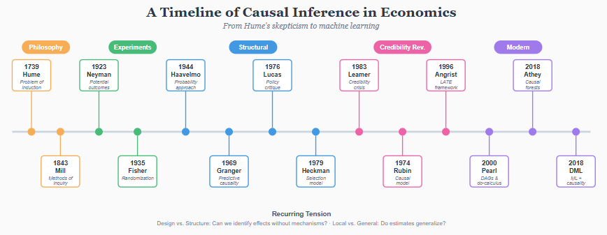
This essay traces how economics came to think about causality. The story involves philosophers, statisticians, econometricians, and computer scientists. It spans three centuries and at least two methodological revolutions. And it remains, in important ways, unfinished.

The philosophical problem: Hume’s challenge

The modern problem of causation begins with David Hume. In A Treatise of Human Nature (1739) and An Enquiry Concerning Human Understanding (1748), Hume posed a question that still has no fully satisfying answer: what do we actually observe when we say that one thing causes another?

Hume’s answer was deflationary. We observe sequences: the flame touches the paper, the paper burns. We observe regularities: flames always burn paper. But we never observe the causation itself-the necessary connection between flame and burning. What we call causation, Hume argued, is just constant conjunction plus a habit of expectation. We see A followed by B repeatedly, and we come to expect B whenever we see A. The “causal power” we attribute to A is a projection of our minds, not a feature of the world.

This matters for empirical research because Hume’s critique applies directly to what we do. We observe that countries with more education have higher GDP. We observe that people who take a drug recover more often. But in neither case do we observe education causing growth or the drug causing recovery. We observe correlations-constant conjunctions-and we want to infer causation.

Hume was not saying causation does not exist. He was saying we cannot perceive it directly. We can only infer it. And inference requires assumptions that go beyond the data.

The entire history of causal inference in statistics and economics can be read as a series of attempts to make those assumptions explicit, testable, or avoidable. Randomization, instrumental variables, potential outcomes, directed acyclic graphs-each approach tries to create conditions under which we can move from observed correlations to causal claims. None escapes Hume’s basic insight: the causal inference always involves something we add to the data, not something the data contains on its own.

The correlation-causation fallacy, both ways

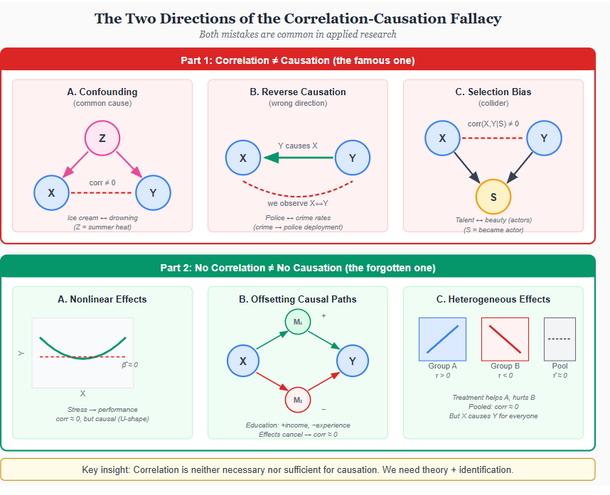
Every student learns that correlation does not imply causation. Few learn the converse: absence of correlation does not imply absence of causation. Both mistakes are common in applied work, and understanding why reveals something fundamental about what causal inference requires.

Why correlation fails to establish causation

The textbook cases are familiar. First, confounding: ice cream sales correlate with drowning deaths not because ice cream causes drowning, but because summer heat increases both. A common cause Z induces correlation between X and Y even when X has no causal effect on Y. Second, reverse causation: neighborhoods with more police have higher crime rates, but this reflects that crime causes police deployment, not the reverse. The direction of causality matters, and correlation alone cannot tell us which way it runs. Third, selection bias: among Hollywood actors, talent and physical attractiveness appear negatively correlated-the “beautiful and dumb” stereotype. But this reflects selection: to become an actor, you need either exceptional talent or exceptional looks (or both). Conditioning on the collider “became an actor” induces a spurious association between its causes.

Each of these failures has a common structure. Correlation measures association-whether knowing X tells you something about Y. Causation asks whether changing X would change Y. These are different questions. Association is symmetric: Corr(X,Y) = Corr(Y,X). Causation is not: X causing Y does not mean Y causes X. Association is about prediction. Causation is about intervention.

The forgotten half: Why absence of correlation fails to rule out causation

The reverse error is less famous but equally important. Finding zero correlation between X and Y does not mean X has no causal effect on Y. Three mechanisms explain why.

Nonlinear effects. If X affects Y through a U-shaped function, the linear correlation can be exactly zero while the causal relationship is strong. Moderate stress improves performance; excessive stress impairs it. Regress performance on stress and you might find nothing. But both low stress and high stress cause lower performance than moderate stress-the relationship is causal, just not linear.

Offsetting paths. X might affect Y through multiple channels that work in opposite directions. Education increases earnings through human capital accumulation (positive), but delays labor market entry and reduces work experience at any given age (negative). If these effects roughly cancel, the correlation between education and earnings at a point in time might be small, even though education causally affects both outcomes. Decomposing total effects into direct and indirect paths requires structural analysis, not just correlation.

Heterogeneous effects. A treatment might help some people and hurt others. If the population is evenly split between those who benefit and those who are harmed, the average effect-and thus the correlation-could be zero. But this does not mean the treatment has no causal effect. It means the effect is heterogeneous. Aggregate correlations can mask causal relationships that operate differently across subgroups.

The deeper lesson

Correlation is neither necessary nor sufficient for causation. You can have correlation without causation (confounding, reverse causation, selection). You can have causation without correlation (nonlinearity, offsetting paths, heterogeneity). The statistical association between X and Y in observational data tells us almost nothing about what would happen if we intervened on X.

This is why causal inference requires more than data. It requires assumptions about how the data were generated-what causes what, what is observed and what is not, what variation is exogenous and what is confounded. These assumptions cannot be tested from data alone. They must be defended with theory, institutional knowledge, and research design.

The first systematic attempts: Mill’s methods

John Stuart Mill, writing in A System of Logic (1843), provided the first systematic framework for causal inference. His “methods of experimental inquiry” remain influential, even if we rarely cite them explicitly.

The Method of Difference is the most important. If we have two situations that are identical in every respect except one-the presence or absence of a potential cause-and we observe different outcomes, then that factor is the cause (or part of the cause) of the difference. This is the logic of the controlled experiment, stated a century before Fisher formalized randomization.

The Method of Agreement works in reverse: if we observe the same outcome in multiple situations that share only one common factor, that factor is likely the cause. The Method of Concomitant Variation notes that if two things vary together-when one increases, the other increases-they are likely causally connected. The Method of Residues subtracts known causes from an effect to isolate what remains.

Mill’s methods have an obvious limitation: they require that we control for, or rule out, all other potential causes. The Method of Difference assumes the two situations differ in only one respect. In practice, situations always differ in multiple ways. We cannot observe the same individual both taking and not taking a drug. We cannot observe the same country both adopting and not adopting a policy.

This is the fundamental problem of causal inference, and Mill’s methods assume it away rather than solve it. The question of how to make valid causal inferences when we cannot hold everything else constant-when we observe either treatment or control, never both-would occupy the next century of methodological work.

The experimental solution: Fisher’s randomization

Ronald Fisher transformed causal inference by shifting the question. Instead of asking how to observe causation, he asked how to create conditions under which correlations reliably indicate causation.

His answer, developed in Statistical Methods for Research Workers (1925) and The Design of Experiments (1935), was randomization. If we randomly assign subjects to treatment and control groups, any pre-existing differences between them are, on average, balanced. The groups differ only in treatment status. Any subsequent difference in outcomes can be attributed to the treatment.

This was a profound insight. Randomization does not require that we know or measure all the confounding factors. It does not require that we understand the mechanism by which treatment affects outcomes. It works, in a sense, despite our ignorance. The design, not the analysis, does the heavy lifting.

Fisher also introduced the idea of the randomization distribution-the distribution of a test statistic under all possible random assignments. This provides the basis for inference without parametric assumptions about the population. If we observe an effect larger than we would expect under random assignment, we conclude that the treatment mattered.

The experimental approach has become the gold standard for causal inference in medicine, psychology, and increasingly in economics. But it has obvious limitations. Many questions of economic interest cannot be randomized. We cannot randomly assign countries to adopt different trade policies. We cannot randomly assign people to different levels of education. And even when randomization is feasible, experiments often study narrow populations in artificial settings, raising questions about whether the results generalize.

Fisher’s contribution was not to solve the problem of causation-Hume’s challenge remains-but to show that clever design can make the problem tractable. The insight that identification comes from design, not from statistical technique applied to observational data, would become central to the credibility revolution decades later.

The forgotten contribution: Neyman’s potential outcomes

The framework that dominates modern causal inference-potential outcomes-was first articulated by Jerzy Neyman in 1923. But his paper was in Polish, published in an agricultural journal, and largely unknown outside a small circle until Donald Rubin rediscovered and extended it in the 1970s.

Neyman’s conceptual move was to define causal effects in terms of hypothetical outcomes. For each unit, there exists a potential outcome under treatment and a potential outcome under control. The causal effect for that unit is the difference between these two potential outcomes.

This framing makes the fundamental problem explicit. We can observe at most one potential outcome for each unit-the one corresponding to whatever treatment the unit actually received. The other potential outcome is counterfactual. It exists conceptually but not observationally. Causal inference, in this view, is the problem of inferring something about unobserved counterfactuals from observed data.

The potential outcomes framework clarifies what we are trying to estimate. The average treatment effect (ATE) is the average difference between potential outcomes across all units. The average treatment effect on the treated (ATT) is the average effect among those who actually received treatment. These are different quantities, and different methods identify different parameters.

Neyman’s framework also clarifies the role of randomization. Under random assignment, the treated and control groups have the same expected potential outcomes in the absence of treatment. Any observed difference in outcomes can therefore be attributed to the treatment effect. Randomization does not eliminate the fundamental problem-we still cannot observe both potential outcomes-but it allows us to estimate average effects by comparing group means.

The potential outcomes framework is sometimes called the Rubin Causal Model, acknowledging Rubin’s role in developing and popularizing it. But the core idea-defining causation in terms of what would have happened under alternative treatments-goes back to Neyman. And this counterfactual conception of causation has deeper roots still, in philosophers like David Lewis who analyzed causation in terms of counterfactual conditionals.

The structural revolution: Haavelmo and the Cowles Commission

While Fisher and Neyman were developing the experimental tradition, a parallel line of work was emerging in economics. This tradition, associated with Trygve Haavelmo and the Cowles Commission, sought to infer causation from observational data using economic theory.

Haavelmo’s 1944 paper “The Probability Approach in Econometrics” marked a turning point. He argued that econometric equations should be interpreted as structural relationships-descriptions of how the economy actually works-not merely as summaries of correlations. The parameters in a supply curve or a production function are causal parameters: they tell us what would happen if we intervened to change one variable.

The Cowles Commission, based at the University of Chicago from 1939 to 1955, developed this vision into a research program. Tjalling Koopmans, Jacob Marschak, and others worked out the conditions under which structural parameters could be identified from observational data. Their answer involved exclusion restrictions: variables that affect one equation but not another. If price affects both supply and demand, we cannot separately identify the two curves from price-quantity data alone. But if we have a variable that shifts supply without affecting demand-a cost shock, say-we can use that variation to trace out the demand curve.

This is the intellectual origin of instrumental variables. An instrument shifts the endogenous variable (price) through a channel (supply) that is excluded from the equation of interest (demand). The exclusion restriction is not testable from the data-it is an assumption derived from economic theory about how the world works.

The structural approach was ambitious. It aimed to estimate complete models of economic systems: supply and demand, production and consumption, savings and investment. With a complete structural model, you could simulate counterfactual policies. What would happen to output if we raised taxes? What would happen to prices if we increased the money supply? The model would tell you.

But this ambition was also the approach’s weakness. The structural models required many assumptions-functional forms, exclusion restrictions, distributional assumptions-that were difficult to defend empirically. And the results were often sensitive to these assumptions in ways that were hard to trace.

The predictive tradition: Granger and temporal causality

While philosophers debated counterfactuals and statisticians developed potential outcomes, a parallel tradition emerged in economics focused on prediction. Clive Granger, working on time series econometrics in the 1960s, proposed a definition of causality that sidestepped metaphysics entirely: X causes Y if past values of X help predict future values of Y, beyond what past values of Y alone can predict.

The intuition is simple. If knowing yesterday’s weather helps me predict today’s crop prices-even after accounting for yesterday’s prices-then weather “Granger-causes” prices. The definition is operational: it tells you exactly what to test. Run a regression of Y on its own lags, then add lags of X. If the X lags are jointly significant, X Granger-causes Y.

Formally, consider two time series X and Y. The standard implementation uses vector autoregressions:

Y_t = α + Σ β_j Y_{t-j} + Σ γ_j X_{t-j} + ε_t

The test for Granger causality is simply whether the γ coefficients are jointly zero.

This approach became enormously influential. The method spread beyond economics into neuroscience (does activity in brain region A precede and predict activity in region B?), climate science, and genomics. It provided a statistical test where other definitions of causality offered only philosophical arguments. Granger later won the 2003 Nobel Prize-though for his work on cointegration with Robert Engle, not for Granger causality-but his concept of predictive causation remains widely used across disciplines.

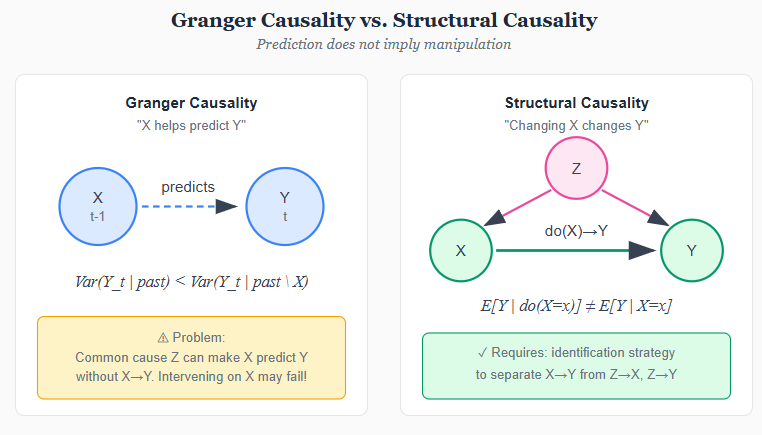
But Granger himself was careful about interpretation. He called his concept “Granger causality” or “G-causality” to distinguish it from causation in the philosophical sense. The definition captures temporal precedence and predictive content, not necessarily mechanism. As critics pointed out, you can construct examples where X Granger-causes Y even though X has no causal influence on Y-common causes, for instance, can create predictive relationships without direct causation.

Holland (1986) drew a sharp distinction. In his taxonomy, Granger causality belongs to a different category than the manipulation-based causality of Rubin and the structural causality of econometrics. Granger causality is about forecasting; the other traditions are about intervention. Knowing that X Granger-causes Y tells you that X is useful for predicting Y. It does not tell you that manipulating X will change Y.

The Granger tradition represents an important fork in the road. One path-the one most of this essay has traced-asks what would happen if we intervened. The other path asks what we can predict. Both are legitimate questions. The danger lies in confusing them: in assuming that predictive relationships license causal claims about intervention.

The Lucas critique: When parameters are not structural

In 1976, Robert Lucas published a paper that would reshape macroeconomics. His target was the large-scale econometric models used for policy evaluation-systems of equations estimated from historical data and then used to simulate the effects of policy changes. Lucas argued that this entire enterprise was fundamentally flawed.

The problem is expectations. Economic agents-households, firms, investors-form expectations about the future and act on them. When policy changes, expectations change. When expectations change, behavior changes. And when behavior changes, the statistical relationships estimated from historical data no longer hold.

Consider the Phillips curve, the empirical relationship between inflation and unemployment that dominated policy discussions in the 1960s. Policymakers observed a trade-off: higher inflation was associated with lower unemployment. They concluded they could exploit this trade-off-accept a bit more inflation to get a bit less unemployment.

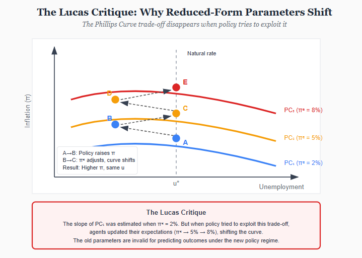
Lucas pointed out the flaw. The historical Phillips curve was estimated under a particular monetary policy regime. Workers and firms had certain expectations about future inflation, and those expectations were embedded in wage contracts, pricing decisions, and investment plans. If policymakers tried to exploit the trade-off by permanently raising inflation, expectations would adjust. Workers would demand higher wages to compensate for expected inflation. Firms would raise prices preemptively. The trade-off would evaporate.

The formal statement is precise. Suppose we estimate a reduced-form relationship:

Y_t = A · X_t + ε_t

where Y is some outcome (unemployment) and X is a policy variable (inflation). The coefficient A summarizes how Y responds to X in historical data. But A is not a “deep” parameter-it depends on expectations, and expectations depend on the policy rule. If we change the policy rule, A changes. Using the old A to predict the effects of a new policy is invalid.

Lucas’s solution was to model the “deep parameters”-preferences, technology, resource constraints-that are genuinely invariant to policy. If you can identify how agents optimize given their environment, you can predict how they will re-optimize when the environment changes. This became the methodological foundation for modern macroeconomics: microfounded models with rational expectations, culminating in the Dynamic Stochastic General Equilibrium (DSGE) framework.

The Lucas critique has implications far beyond macroeconomics. Any time we use historical relationships to predict the effects of a new policy, we face the same problem. Will the estimated effect of a job training program persist if we scale it up? Will the price elasticity estimated under one tax regime hold under another? Will the relationship between advertising and sales survive a change in competitive strategy?

These questions connect directly to external validity. The critique says that reduced-form estimates-even causally identified ones-may not be policy-invariant. A valid LATE tells you the effect for compliers induced by a particular instrument under a particular policy regime. Change the regime, and the compliers may respond differently.

The structural tradition in economics can be read as a long response to the Lucas critique. If reduced forms are unstable, estimate structure. If behavior depends on expectations, model expectations explicitly. If parameters shift with policy, identify the parameters that do not shift.

The credibility revolution largely set these concerns aside. The focus on design and local identification bracketed questions about structural stability and policy extrapolation. But the critique never went away. It resurfaces whenever we ask whether experimental results generalize, whether estimates from one context apply to another, or whether predictions based on historical data will hold in a changed policy environment.

The crisis of credibility: Leamer and “con out of econometrics”

By the 1970s, structural econometrics was under attack. The critique came from multiple directions, but Edward Leamer’s 1983 article “Let’s Take the Con out of Econometrics” crystallized the concern.

Leamer’s point was simple and devastating: econometric results depend on specification choices that are rarely justified and often not even reported. The same data can support wildly different conclusions depending on which control variables you include, which functional form you assume, and which observations you exclude. In Leamer’s words, “the mapping from data to conclusions is many-to-many.”

He demonstrated this with a reanalysis of a study on capital punishment and murder rates. By varying the specification within reasonable bounds, he could produce estimates ranging from a large deterrent effect to a large increase in murders. The original study’s conclusion was not robust-it was an artifact of one particular specification among many.

Christopher Sims, in his 1980 critique of structural models, raised related concerns. The exclusion restrictions that identified structural parameters were “incredible”-they relied on theoretical distinctions (this variable affects supply but not demand) that could not be tested and often seemed arbitrary. Sims advocated for vector autoregressions (VARs), which imposed minimal structure and “let the data speak.”

The crisis of credibility was not about statistical technique. It was about the gap between the assumptions required for causal inference and the evidence available to support those assumptions. Structural econometrics claimed to identify causal parameters, but the identifying assumptions were built on faith in economic theory, and reasonable people could disagree about the theory.

The response would come in two forms. One was to be more honest about uncertainty-to report sensitivity analyses, to acknowledge that results depend on assumptions. The other was to find designs where the identifying assumptions were more credible. The second response became the credibility revolution.

The Rubin framework: Formalizing potential outcomes

Donald Rubin’s work in the 1970s and 1980s brought potential outcomes to the center of causal inference. His papers-”Estimating Causal Effects of Treatments in Randomized and Nonrandomized Studies” (1974), “Assignment to Treatment Group on the Basis of a Covariate” (1977), and “Bayesian Inference for Causal Effects” (1978)-established the framework that most applied researchers now use, often without knowing its source.

Rubin’s framework unifies experimental and observational studies under the same conceptual structure. In both cases, we have potential outcomes Y(1) and Y(0) for each unit. In an experiment, random assignment ensures that treatment is independent of potential outcomes-the unconfoundedness assumption holds by design. In an observational study, we need to assume unconfoundedness conditional on observed covariates: given what we observe about a unit, its treatment status is as good as random.

This assumption-sometimes called “selection on observables”-is strong. It says that we have measured everything that jointly affects treatment and outcome. There is no unmeasured confounding. Whether this is plausible depends entirely on the substantive context. In some settings, we have rich data and strong reasons to believe we have captured the relevant differences. In others, the assumption is clearly untenable.

Rubin also formalized the Stable Unit Treatment Value Assumption, or SUTVA. This assumption says that a unit’s potential outcomes depend only on its own treatment status, not on which other units are treated. There is no interference between units, and there is only one version of treatment. These assumptions rule out spillovers, general equilibrium effects, and treatment heterogeneity of certain kinds. They are often violated in economic settings, and violations complicate both estimation and interpretation.

The Rubin Causal Model provides a common language for discussing causal inference. It makes assumptions explicit. It clarifies what we are estimating (average effects, effects on the treated, local effects). And it separates identification-what we could learn with infinite data-from estimation-how we learn it from finite samples. This conceptual clarity was one of the framework’s most important contributions.

`The credibility revolution: Design over structure

The 1990s brought a transformation in how economists approach causal inference. Joshua Angrist, Guido Imbens, and their collaborators developed methods-and perhaps more importantly, a methodological philosophy-that prioritized transparent identification over structural modeling.

The key papers include Angrist and Krueger on compulsory schooling laws (1991), Card on the Mariel boatlift (1990), and the Angrist-Imbens-Rubin paper on local average treatment effects (1996). Each exploited a natural experiment or quasi-experimental variation to identify causal effects without relying on elaborate structural models.

The LATE framework was particularly influential. Angrist and Imbens showed that when you use an instrumental variable, you identify the average effect for a specific subpopulation: the compliers, who change their treatment status in response to the instrument. You do not identify the effect for always-takers, never-takers, or defiers. The estimate is local to the compliers induced by your particular instrument.

This was both clarifying and sobering. Different instruments identify different parameters, even for the same treatment. The return to education estimated using Vietnam draft lottery variation applies to men who would have attended college if not drafted but stayed home otherwise. It does not necessarily apply to people who always go to college regardless, or who never go regardless. If we want to know the effect for a different population, we need either a different instrument or additional assumptions.

The credibility revolution shifted the profession’s focus from structure to design. What matters is not the sophistication of your model but the plausibility of your identifying variation. A simple comparison of means, with credible random assignment, beats a complex structural model with doubtful exclusion restrictions. Angrist and Pischke’s Mostly Harmless Econometrics (2009) codified this approach for a generation of applied researchers.

The shift had costs as well as benefits. Emphasizing design over structure sometimes meant ignoring mechanisms, discounting theory, and settling for narrow answers to narrow questions. Critics-including James Heckman-argued that the credibility revolution had gone too far, substituting methodological purity for economic substance. This debate continues.

The outsider: Pearl and the graphical approach

While economists were developing the potential outcomes framework and the design-based approach, Judea Pearl was building a different foundation for causal inference. A computer scientist at UCLA, Pearl approached causation through directed acyclic graphs (DAGs) and the “do-calculus.”

Pearl’s framework starts with a causal graph: a diagram showing which variables directly affect which other variables. An arrow from X to Y means X is a direct cause of Y. A path from X to Y through intermediate variables represents an indirect effect. The graph encodes qualitative assumptions about causal structure.

The key innovation is the distinction between seeing and doing. Observing that X and Y are correlated tells us something different from intervening to change X and seeing what happens to Y. The conditional distribution P(Y|X) is not the same as the interventional distribution P(Y|do(X)). Confounding creates the gap: when a third variable affects both X and Y, observing high X values might predict high Y values even if manipulating X would have no effect.

The do-calculus provides rules for translating between observational and interventional distributions. Given a causal graph and observational data, the rules tell you whether and how you can identify causal effects. The backdoor criterion identifies when conditioning on a set of variables blocks all confounding paths. The front-door criterion shows that you can sometimes identify effects even with unmeasured confounding, if you observe the right intermediate variables.

Pearl has been critical of the potential outcomes framework, arguing that it lacks a formal language for representing causal structure. In his view, writing down potential outcomes is not enough; you need to specify which variables affect which. The graph makes assumptions explicit in a way that potential outcomes alone do not.

Economists have been slow to adopt Pearl’s framework, for reasons both substantive and sociological. The graphical approach is less familiar. The vocabulary is different. And some economists worry that drawing a DAG creates false confidence-the graph looks precise, but the arrows represent assumptions that may or may not hold.

Still, the graphical approach has made inroads. It provides a systematic way to think about identification, to diagnose confounding, and to analyze complex causal structures. For problems like mediation analysis or selection bias, DAGs offer clarity that algebraic approaches lack.

The Heckman response: Structure strikes back

James Heckman has been the most prominent defender of the structural tradition against the design-based revolution. His critique operates on several levels.

First, Heckman emphasizes that LATE is not ATE. The local average treatment effect applies to compliers induced by a particular instrument. It does not apply to the entire population, and it may not even apply to the population affected by a proposed policy. If we want to know what would happen if we expanded a program, we need to know effects for marginal participants-who may differ from the compliers induced by historical variation.

The Marginal Treatment Effects framework addresses this concern. MTE estimates the treatment effect at each point along the distribution of unobserved resistance to treatment. From the MTE curve, you can compute any treatment effect parameter-ATE, ATT, LATE, or policy-relevant treatment effects-by integrating with appropriate weights. Different instruments identify different weighted averages of the same underlying MTE curve.

Second, Heckman argues that identification without structure is often impossible. The design-based approach works well when you have a clean natural experiment. But many important questions-effects of education, effects of job training, effects of macroeconomic policies-do not come with clean instruments. Understanding mechanisms and imposing structure, judiciously, may be the only way forward.

Third, Heckman emphasizes heterogeneity. People differ in their responses to treatment, and this heterogeneity is often systematic. Those who choose treatment may do so because they expect to benefit. Ignoring this selection on gains gives misleading estimates of policy effects. Structural models that explicitly model selection can recover the full distribution of effects, not just an average.

The debate between design-based and structural approaches is not resolved. Each tradition has strengths. Design-based methods offer transparency and credibility when good designs exist. Structural methods offer flexibility and policy relevance when they do not. The best work often combines both-using quasi-experimental variation to identify structural parameters, or using structure to interpret and extrapolate quasi-experimental estimates.

The present: Synthesis and new frontiers

Contemporary causal inference draws on all these traditions. The conceptual vocabulary comes from Rubin’s potential outcomes. The emphasis on design comes from Angrist and the credibility revolution. The language of graphs and identification comes from Pearl. The attention to heterogeneity and policy relevance comes from Heckman.

Several frontiers are active.

Synthetic control methods, introduced by Abadie and Gardeazabal (2003) and formalized by Abadie, Diamond, and Hainmueller (2010), provide a way to construct counterfactuals for single treated units. When you want to know what would have happened to California without Proposition 99 or to Germany without reunification, you cannot run an experiment. Synthetic control builds a weighted comparison from untreated units, trading randomization for data-driven matching.

Difference-in-differences has undergone a methodological renaissance. The method’s intellectual roots reach back further than most economists realize - to the 1840s and 1850s. In 1847, Ignaz Semmelweis used comparative clinic analysis to show that handwashing prevented childbed fever, comparing mortality between Vienna’s physician-staffed ward (where medical students performed autopsies) and its midwife-staffed ward, then tracking outcomes after implementing chlorine disinfection. John Snow’s 1854 investigation of cholera in London is credited as the first recorded application of difference-in-differences proper. Snow compared mortality rates across households served by two water companies: the Lambeth Company, which had moved its intake upstream of the city’s sewage outflow in 1852, and the Southwark & Vauxhall Company, which continued drawing contaminated water. By comparing changes in cholera deaths before and after Lambeth’s relocation - while Southwark & Vauxhall served as the control - Snow produced a cleaner diff-in-diff design, with parallel pre-treatment trends giving way to dramatic divergence. His “Grand Experiment” found 315 deaths per 10,000 households among Southwark & Vauxhall customers versus only 37 per 10,000 among Lambeth customers, providing powerful evidence for the waterborne transmission of cholera decades before germ theory was established.

More recently, work by Goodman-Bacon, Callaway and Sant’Anna, de Chaisemartin and D’Haultfœuille, and others has clarified what two-way fixed effects actually estimate when treatment timing varies and effects are heterogeneous. The answers were often not what applied researchers assumed. New estimators address the problems, but they also require more from the data and from the researcher.

The external validity problem-whether effects estimated in one context generalize to another-has become central. Transportability theory, developed by Pearl and Bareinboim, provides formal conditions under which results can be extrapolated across populations. Applied researchers increasingly worry about whether their local estimates tell us anything about the settings policymakers care about. The credibility revolution, focused on internal validity, deferred this question. It is now returning with force.

AI and the future of causal inference

The past decade has seen an explosion of work at the intersection of machine learning and causal inference. The contributions operate at different levels-from automating routine tasks to potentially addressing fundamental problems that have resisted solution for decades.

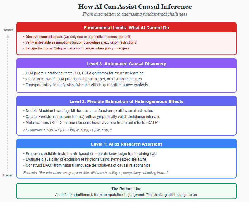
Level one: AI as research assistant

At the most basic level, large language models can function as automated domain experts. Identifying valid instruments has always required substantive knowledge: what variables affect treatment but not outcome except through treatment? Traditionally, researchers relied on intuition, literature review, and consultation with experts. LLMs can accelerate this process.

Given a treatment and outcome, an LLM can propose candidate instruments, assess the plausibility of exclusion restrictions, and flag potential violations. “For estimating returns to education, consider: compulsory schooling laws, distance to colleges, birth quarter interacted with school entry cutoffs...” The suggestions are not infallible, but they provide a starting point that previously required hours of literature search.

Similarly, LLMs can help construct causal graphs. Given a description of variables and their relationships, they can propose directed acyclic graphs encoding assumed causal structure. Several frameworks now combine LLM-generated graphs with statistical tests for conditional independence, iteratively refining the structure based on data.

The value here is not that AI solves the identification problem. It is that AI reduces the friction in applying domain knowledge. The bottleneck in causal inference has always been the gap between data and assumptions. AI cannot eliminate the need for assumptions, but it can help researchers articulate and scrutinize them.

Level two: Flexible estimation of heterogeneous effects

A deeper contribution involves estimation. Traditional methods for causal inference-regression, matching, instrumental variables-require the researcher to specify functional forms. Which variables to control for, how they enter the model, whether effects vary with covariates. These choices matter, and getting them wrong introduces bias.

Machine learning offers an alternative: let the data determine functional form. Double Machine Learning, developed by Chernozhukov and colleagues, provides a framework for this. The key insight is that estimating a causal parameter often involves two estimation problems: predicting the outcome given covariates, and predicting treatment given covariates. If these “nuisance functions” are estimated flexibly-with random forests, neural networks, or any ML method-the resulting causal estimate remains valid, provided certain orthogonality conditions hold.

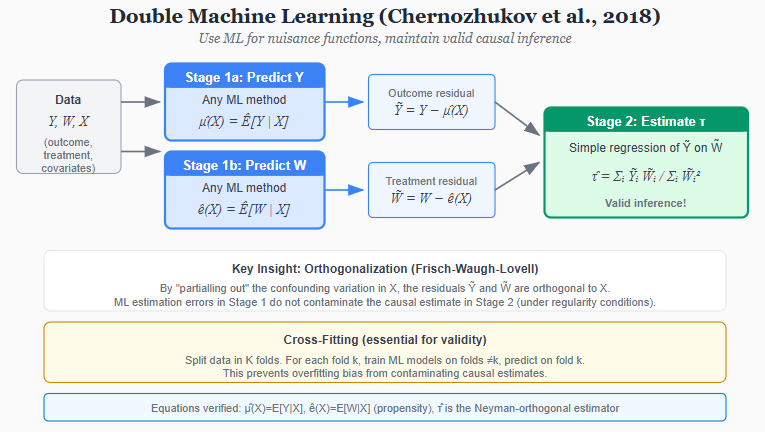
The procedure has two stages. First, use ML to predict Y from X (the covariates) and to predict treatment W from X. These predictions partial out the confounding variation. Second, estimate the causal effect from the residualized relationship. The formula is elegant:

τ = E[(Y - μ̂(X))(W - ê(X))] / E[(W - ê(X))²]

where μ̂(X) is the predicted outcome and ê(X) is the predicted treatment probability (propensity score). The cross-fitting procedure ensures that the ML estimation error does not contaminate the causal estimate.

Causal forests, developed by Athey and Wager, go further. Rather than estimating a single average effect, they estimate how effects vary across individuals. The algorithm partitions the covariate space to find regions where treatment effects are approximately constant, then estimates effects within each region. The result is a fully nonparametric estimate of τ(x)-the treatment effect as a function of observable characteristics-with valid confidence intervals.

These methods transform what is possible. Questions that previously required strong parametric assumptions-does the effect of a drug vary with age? does job training work better for some workers than others?-can now be addressed flexibly. The researcher specifies the causal framework (what is the treatment, what confounders must be controlled), and the algorithm handles the functional form.

Level three: Causal discovery from text and knowledge

The most ambitious applications involve causal discovery-learning causal structure from data, potentially augmented with prior knowledge encoded in language models.

Traditional causal discovery algorithms like PC and FCI use conditional independence tests to infer which variables directly cause which. These methods require observed data on all relevant variables and strong assumptions about the data-generating process. In practice, they often produce graphs riddled with undetermined edges.

LLMs offer a new input: prior knowledge at scale. An LLM trained on scientific literature has absorbed millions of causal claims-”smoking causes cancer,” “interest rates affect investment,” “rainfall influences crop yields.” This knowledge is noisy and sometimes wrong, but it is vast. Recent work combines LLM-generated priors with statistical tests, using the LLM to propose edges and the data to verify or refute them.

Whether this approach can scale to complex economic and social systems remains to be seen. The causal relationships in economics are often subtle, contested, and context-dependent. An LLM might correctly identify that “education affects earnings” while missing the endogeneity that makes this relationship so hard to estimate. The technology is promising but immature.

The fundamental limits

What AI cannot do is resolve the fundamental problem of causal inference. We still observe only one potential outcome per unit. We still cannot directly test the assumptions-unconfoundedness, exclusion restrictions, SUTVA-that license causal interpretation. We still face the Lucas critique: the relationships we estimate may not survive changes in policy.

AI offers scale, flexibility, and automation. It can explore heterogeneity that would be invisible to parametric methods. It can synthesize domain knowledge that would take humans weeks to compile. It can fit complex functional forms without researcher specification.

But the core challenge remains what it has been since Hume: causation is not observed, only inferred. The inference requires assumptions that cannot be verified from data alone. No amount of computational power changes this. The researcher must still defend why the instrument is valid, why unobserved confounding is absent, why the estimate generalizes.

The optimistic view is that AI shifts the bottleneck. If the hard part of causal inference is articulating and checking assumptions, AI can help. If the hard part is estimating flexibly in high dimensions, AI can help. If the hard part is synthesizing evidence across contexts, AI can help.

The pessimistic view is that AI makes it easier to produce causal claims and harder to evaluate them. Automated pipelines can generate estimates at scale, but can they generate wisdom about when those estimates are trustworthy? The history of econometrics suggests that methodological advances often outpace the understanding needed to apply them responsibly.

The honest view is probably somewhere between. AI is a tool-powerful, rapidly improving, but still a tool. It does not answer the question of what causes what. It helps us formulate and test our answers. The thinking still belongs to us.

What we learned and what remains

The history of causal inference is a history of making assumptions explicit. Hume showed that causation cannot be directly observed-we can only infer it. Every method since has been a proposal for what to assume and what to conclude.

Fisher and Neyman showed that randomization could eliminate confounding, allowing causal inference without knowing the mechanism. But experiments are not always feasible, and experimental results do not always generalize.

The structural tradition showed that economic theory could fill the gap, allowing causal inference from observational data. But the identifying assumptions were often incredible, and results were sensitive to untestable specifications.

The credibility revolution showed that natural experiments and quasi-experimental designs could provide credible identification without elaborate structure. But design-based estimates are often local, and the populations they inform may not be the populations we care about.

Pearl showed that graphical models could make causal structure explicit and provide a calculus for identification. But the graphs encode assumptions that cannot be verified from the data.

Heckman showed that heterogeneity matters-that treatment effects vary, that selection is systematic, and that policy-relevant parameters may differ from what simple designs identify. But the methods that address heterogeneity require structure, and structure requires assumptions.

Each tradition contributes something. None solves the problem completely. The question is not which approach is correct but which assumptions are defensible in a given context. Transparency about those assumptions-what we are claiming, what we are taking on faith-is the common thread.

Three tensions run through this history and remain unresolved.

First: does causal inference require understanding mechanisms, or can we black-box them? The experimental and design-based traditions say we can identify effects without knowing why they occur. The structural tradition says that understanding mechanisms is essential for prediction and policy. Both have a point. Knowing that a drug works matters even if we do not know the biochemistry. But knowing the biochemistry matters if we want to design better drugs.

Second: what is “the” causal effect? The potential outcomes framework defines individual-level effects, but we can rarely estimate them. We estimate averages-ATE, ATT, LATE-which aggregate over heterogeneous individuals. Different methods estimate different averages. The MTE framework shows these are all weighted integrals of the same underlying curve, but that curve itself is an abstraction. Effects are local to populations, contexts, and moments. Speaking of “the effect of education” may be a category error.

Third: what does it mean for results to generalize? A well-identified estimate tells us what happened in one place at one time. Whether it applies elsewhere is a different question-one that our methods for internal validity do not answer. The gap between what we can credibly estimate and what we want to know for policy is real. Filling that gap requires assumptions about mechanisms, about context, about the conditions under which effects persist. Those assumptions rarely have the same epistemic status as a good randomized trial.

Some worth readings

Philosophical Foundations

Hume, David. 1739. A Treatise of Human Nature. - Where causality skepticism begins. Hume’s argument that we never observe causation directly, only constant conjunction, haunts every causal inference we attempt.

Mill, John Stuart. 1843. A System of Logic. - Codifies the methods of agreement, difference, and concomitant variation. Still the intuitive basis for how most scientists think about establishing causation.

Historical Precursors

Semmelweis, Ignaz. 1861. Die Ätiologie, der Begriff und die Prophylaxis des Kindbettfiebers [The Etiology, Concept, and Prophylaxis of Childbed Fever]. Pest: C.A. Hartleben. - Comparative clinic analysis that pioneered systematic before-after comparison with control groups. Showed handwashing prevented childbed fever decades before germ theory.

Snow, John. 1855. On the Mode of Communication of Cholera. 2nd ed. London: John Churchill. - The first recorded difference-in-differences analysis. Snow’s “Grand Experiment” comparing London water companies remains a model of natural experiment design.

Experimental Design & Statistical Foundations

Fisher, Ronald A. 1935. The Design of Experiments. Oliver and Boyd. - Establishes randomization as the gold standard. The lady tasting tea and the principles of experimental design that launched modern statistics.

Holland, Paul W. 1986. “Statistics and Causal Inference.” Journal of the American Statistical Association 81(396): 945-960. - “No causation without manipulation.” Crystallizes the potential outcomes framework and its philosophical commitments. Essential for understanding what the Rubin causal model can and cannot do.

The Structural Econometrics Tradition

Haavelmo, Trygve. 1944. “The Probability Approach in Econometrics.” Econometrica 12(Supplement): iii-vi, 1-115. - The manifesto for structural econometrics. Introduces the crucial distinction between prediction and policy evaluation that still divides the field.

Granger, Clive W.J. 1969. “Investigating Causal Relations by Econometric Models and Cross-spectral Methods.” Econometrica 37(3): 424-438. - Defines predictive causality for time series. Controversial but influential - a pragmatic alternative to structural approaches.

Lucas, Robert E. 1976. “Econometric Policy Evaluation: A Critique.” Carnegie-Rochester Conference Series on Public Policy 1: 19-46. - The critique that changed macroeconomics. Shows why reduced-form relationships break down under policy interventions when agents are forward-looking.

Heckman, James J., and Edward Vytlacil. 2005. “Structural Equations, Treatment Effects, and Econometric Policy Evaluation.” Econometrica 73(3): 669-738. - The definitive integration of structural and treatment effects approaches. Shows how LATE, ATE, and ATT are all weighted averages of the marginal treatment effect. Technical but essential.

Heckman, James J. 2010. “Building Bridges Between Structural and Program Evaluation Approaches to Evaluating Policy.” Journal of Economic Literature 48(2): 356-398. - Heckman’s attempt at reconciliation between the warring camps. Argues both traditions have something to offer and neither alone is sufficient.

The Potential Outcomes Framework

Rubin, Donald B. 1974. “Estimating Causal Effects of Treatments in Randomized and Nonrandomized Studies.” Journal of Educational Psychology 66(5): 688-701. - Introduces the potential outcomes notation that would become ubiquitous. Deceptively simple formalism with profound implications.

Angrist, Joshua D., Guido W. Imbens, and Donald B. Rubin. 1996. “Identification of Causal Effects Using Instrumental Variables.” Journal of the American Statistical Association 91(434): 444-455. - Defines LATE and the complier framework. Clarifies exactly what IV estimates and for whom. The paper that made economists honest about external validity.

Imbens, Guido W., and Donald B. Rubin. 2015. Causal Inference for Statistics, Social, and Biomedical Sciences. Cambridge University Press. - The comprehensive textbook treatment of potential outcomes. Rigorous and thorough; the reference for design-based causal inference.

The Credibility Revolution

Leamer, Edward E. 1983. “Let’s Take the Con out of Econometrics.” American Economic Review 73(1): 31-43. - The wake-up call. Documents how researchers’ prior beliefs determine their conclusions, even with the same data. Demanded transparency that took decades to arrive.

Angrist, Joshua D., and Alan B. Krueger. 1991. “Does Compulsory School Attendance Affect Schooling and Earnings?” Quarterly Journal of Economics 106(4): 979-1014. - Quarter of birth as an instrument for schooling. A template for the natural experiments approach, though later scrutinized for weak instruments.

Angrist, Joshua D., and Jorn-Steffen Pischke. 2009. Mostly Harmless Econometrics: An Empiricist’s Companion. Princeton University Press. - The credibility revolution’s handbook. Regression, IV, diff-in-diff, and RD explained with clarity and attitude. Shaped how a generation thinks about causal inference.

Athey, Susan, and Guido W. Imbens. 2017. “The State of Applied Econometrics: Causality and Policy Evaluation.” Journal of Economic Perspectives 31(2): 3-32. - A survey of where the field stands. Accessible overview of modern methods and their limitations.

Causal Graphs & Structural Causal Models

Pearl, Judea. 2009. Causality: Models, Reasoning, and Inference. 2nd ed. Cambridge University Press. - The alternative paradigm. DAGs, do-calculus, and a framework for reasoning about causation that has slowly penetrated economics. Essential for understanding confounding, mediation, and identification.

Machine Learning & Causal Inference

Athey, Susan, and Stefan Wager. 2018. “Estimation and Inference of Heterogeneous Treatment Effects Using Random Forests.” Journal of the American Statistical Association 113(523): 1228-1242. - Causal forests for treatment effect heterogeneity. Shows how to adapt ML methods to estimate who benefits most from treatment, with valid inference.

Chernozhukov, Victor, et al. 2018. “Double/Debiased Machine Learning for Treatment and Structural Parameters.” The Econometrics Journal 21(1): C1-C68. - How to use ML for nuisance parameters while preserving valid inference for causal effects. The technical foundation for combining flexibility with rigor.