On Good (Bad) Controls
Good controls can move your estimate, Bad controls can leave it unchanged

When a coefficient barely moves after you pile in a set of controls, what has it actually shown?
Suppose you present a baseline regression in a presentation, the coefficient on X that the paper is about, and a commentator ask whether it holds up once you control for things. Covariates go in, the coefficient stays put, and the result “survives.”
The ritual, as it is usually run, shows close to nothing. Robustness checks are useful. The problem is the sentence attached to them. “The coefficient is stable when I add controls” sounds like a statement about whether an estimate is credible. Some people even would claim causality. But, actually it is a statement about something else, and the distance between the two is where applied work goes quietly wrong.
The claim, stated plainly:
Coefficient movement is not a diagnostic of whether a control is good. It only records how the regression, and what it estimates, change once you condition.
Three consequences follow, and they are the whole essay:
A good control can move the coefficient a lot.
A bad control can move the coefficient very little.
Coefficient stability is not identification.
The literature has a name for part of this, “bad controls,” though the classroom shorthand often hides more than it shows. What follows is an attempt to untangle it. I find this worthy because I have had this issue before in my own work.
Two reasons we add controls
Two separate questions hide inside any decision to include a covariate W. The first is structural. Does conditioning on W help recover the causal effect of X on Y? This is a question about the data-generating process, about which arrows point where, and it has the same answer in a sample of fifty or fifty million. The second is statistical. When W enters this regression, does β move, and by how much? This one is about the correlations in the sample at hand.
The structural question is whether conditioning changes the causal object being estimated. The statistical question is how much the coefficient changes in this particular sample. The first is answered by assumptions. The second is answered by algebra. The regression table can answer the second. It cannot touch the first.
Applied work runs the two together. Controls go in “to see if the result holds,” the coefficient’s movement gets read as a signal about whether those controls belonged, and a steady estimate passes for a clean bill of health. The questions are independent, though. A control can be the right thing to include and still swing the coefficient hard, which is what a confounder does once it is finally adjusted for. A control can wreck identification and leave the estimate almost untouched.
First, then, the structural picture.
A taxonomy of controls
Causal diagrams make the structural question concrete. That’s the reason I find very useful DAGs. The back-door criterion is the working rule: to identify the effect of X on Y, every non-causal path between them has to be blocked, without opening a new one and without blocking the causal path. Whether a given W helps depends on where it sits.
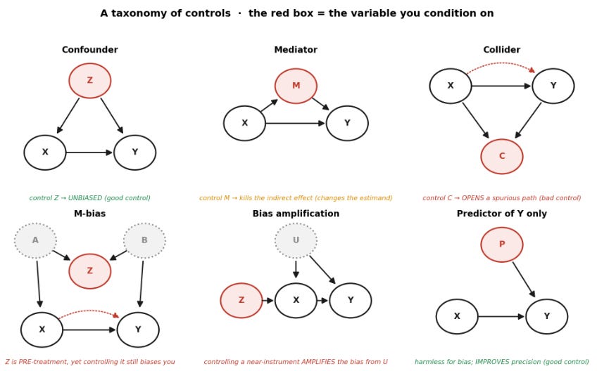
The six cases. The red node is the variable being conditioned on. Solid arrows are causal. The dashed red arc is the spurious association that conditioning opens up.
What conditioning does in each case:
Confounder. Z causes both X and Y, so it sits on the back-door path X ← Z → Y. Adjusting for it is correct, the textbook good control.
Mediator. M sits on the causal channel itself, X → M → Y. Conditioning on it strips out the part of the effect that runs through M. That can be appropriate if the estimand is a controlled direct effect, but it is no longer the total effect, and most papers that do it are still reporting the total.
Collider. C is a common effect of X and Y. Left alone it blocks a spurious path. Conditioning on it opens a path that was closed, inventing an association between X and Y. The canonical bad control.
M-bias. The case that trips people up. In the canonical M-structure, Z comes before X in time, yet it is a collider on a path running through two unobserved causes, so adjusting for it biases the estimate anyway. The rule “control for anything measured pre-treatment” does not hold.
Bias amplification. Z behaves like an instrument: it moves X and reaches Y only through X. When there is unmeasured confounding U, adding Z leaves the bias in place and makes it bigger. The mistake is not that instruments are bad. It is treating an instrument-like variable as an ordinary control in a confounded OLS regression, which is a different thing from using it as an instrument in IV.
Predictor of Y only. P affects Y but not X, so it cannot confound the relationship. It is not needed for identification, but it soaks up residual variance and improves efficiency. A good control, for a reason that has nothing to do with bias.
The lesson is not that controls are good or bad by nature. The same act, conditioning, can block confounding, block the causal effect, open a collider path, amplify existing bias, or improve precision. The full catalog is in Cinelli, Forney, and Pearl (2024). The point that collider, confounding, and overcontrol bias are three distinct problems is Elwert and Winship (2014). The pre-treatment version that ruins experiments is Montgomery, Nyhan, and Torres (2018), after Rosenbaum (1984).
The same move, three meanings
Take three simulated worlds where the true effect of X on Y is known. In each, the regression runs with and without “the control.”
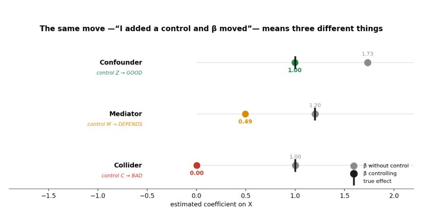
Confounder world. True effect 1.0. Without the control the estimate is 1.73, biased upward because the omitted Z drives both variables. Add Z and it lands at 1.00. The control corrected it.
Mediator world. Total effect 1.2. Without the control the estimate is 1.20, which is right when the total effect is the target. Add the mediator and it drops to 0.49. No bias was removed. The estimand changed.
Collider world. True effect 1.0. Without the control the estimate is already 1.00. Add the collider and it falls to 0.00. Conditioning broke an estimate that started out correct.
Every time, β̂ moved when a control went in. The first movement was the control doing its job. The second was a change of estimand presented as a robustness check. The third was bias created out of thin air. The magnitude and direction say nothing about which of the three it was.
Stated plainly: the movement of β̂ does not diagnose whether W belongs in the regression. It records what happened after conditioning. If W is a confounder, movement may be the correction of bias. If W is a mediator, movement may be a change in the estimand. If W is a collider, movement may be bias the regression manufactured. And if the coefficient barely moves, none of this is settled. A bad control can be quiet. A good control can be loud.
That last point is the one the three-cases picture cannot show on its own. The full grid can. Columns are how much the coefficient moves. Rows are whether the control is good or bad. All four cells exist.
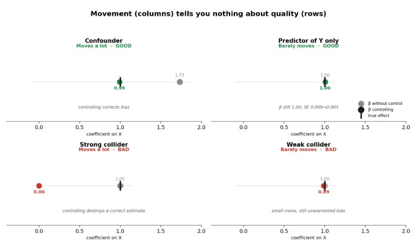
Top row, two good controls: the confounder swings the estimate from 1.73 to 0.99, while a pure predictor of Y leaves β̂ at 1.00 and just halves the standard error. Bottom row, two bad controls: the strong collider crashes the estimate to 0.00, while a weak collider nudges it from 1.00 to 0.99. The bottom-right cell is the dangerous one: a 1% move reads as “robust,” and the control is still illegitimate. Stability did not rescue it.
The collider mechanism is the hardest to believe the first time, so it earns its own picture. Consider two independent variables, talent and beauty, and a third that both of them cause, like making a living as an actor. In the whole population talent and beauty are uncorrelated. Restrict to working actors and a negative correlation appears: among the people who made it, someone short on talent has to be unusually good-looking to have gotten there, and the other way around.
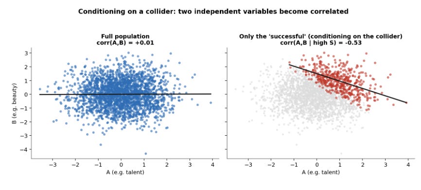
+0.01 in the full population, −0.53 once the collider is conditioned on. The variables did not change. Selecting on the collider did all of it.
The actor story is toy language for a problem that turns up constantly: conditioning on admission, survival, employment, program take-up, presence in the administrative records, or any sample restriction defined after treatment. Each of those conditions on a collider, and the bias is baked into the sample before a model runs.
The robustness ritual, and where Gelbach comes in
Coefficient movement, then, does not reveal whether a control belongs. A quieter problem waits even when every control does belong, in a clean confounding world where adjusting is the right call. The usual way of reporting the movement still does not hold together.
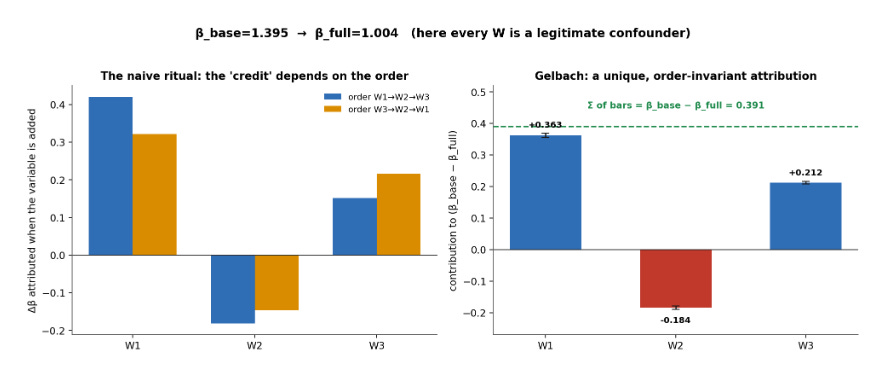
The ritual runs like this: a regression of Y on X, then controls added one at a time, with the path of the coefficient narrated. “It drops forty percent with demographics, then settles.” The catch is that when controls are correlated with each other, the incremental contribution of each one depends on the order they enter. Whichever control goes in first gets the credit. The same control entered last, after the others have absorbed the shared variation, looks inert. Same variables, same data, a story set by typing order.
Jonah Gelbach settled this in “When Do Covariates Matter? And Which Ones, and How Much?” (Journal of Labor Economics, 2016). The fix falls out of the omitted-variables-bias formula. The full model is
Omit the Wₖ and the short-regression coefficient is
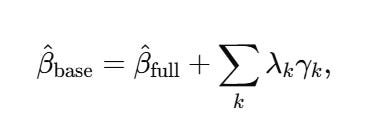
where, in the simplest one-treatment case, λₖ is the slope from regressing the covariate Wₖ on X alone, and γₖ is its coefficient in the full model. (With baseline controls, fixed effects, or weights, the same logic runs on residualized regressions.) Each product λₖ γₖ is control k’s contribution to the gap between the base and full estimates. Because λₖ uses the unconditional auxiliary regression and γₖ comes from the full model, the decomposition is unique, it ignores entry order, and the pieces sum to β̂_base − β̂_full.
The right panel shows it. β̂_base = 1.395 falls to β̂_full = 1.004, a gap of 0.391. Gelbach assigns +0.363 of it to W₁, −0.184 to W₂, and +0.212 to W₃, and those add up to 0.391 to within floating-point error. (The decomposition also nests the Oaxaca and Blinder decomposition and extends to IV. Gelbach derives the standard errors, and the bars carry bootstrap intervals.)
That answers “which controls move the coefficient, and by how much.” It removes the order dependence and gives every covariate a fair share. It decomposes the gap between the short and long regression, nothing more.
And here is the limit. Every Wₖ in this simulation is a real confounder. The decomposition reports how much each one moved β̂ and says nothing about whether moving β̂ was warranted.
A note on that claim. It is the unconditional one. Without knowing a control’s structural role, the size of the movement does not reveal whether conditioning helped or hurt. Conditional on already knowing that W is a legitimate confounder, the magnitude is informative: a large move signals severe confounding, which is exactly what Oster’s bound exploits. What carries no structural information is the movement taken on its own.
Pointed at the collider world, the same machinery reports how much the collider “explains,” handing back a bias dressed as an explanation. Gelbach answers the statistical question with precision. The structural question, whether a variable is a confounder to adjust for or a collider that is fooling you, is not in the data and never will be. It comes from the diagram. (This is separate from the high-dimensional selection problem of Belloni, Chernozhukov, and Hansen (2014): machine learning can choose which predictors to keep, but it cannot decide whether a variable is a confounder, a mediator, or a collider.)
The honest version of “is it stable?”
If coefficient stability is to carry weight, say as an argument that unmeasured confounding is unlikely to flip a result, there is a disciplined way to make the case. It is Oster’s (Journal of Business & Economic Statistics, 2019), building on Altonji, Elder, and Taber (2005). The idea: if selection on observables runs proportional to selection on unobservables, then coefficient movement together with R² movement, as controls are added, bounds the bias from what went unmeasured.
In a simulation with one confounder left unobserved, the estimate moves from 1.89 with no controls to 1.57 with the observed ones. Oster’s logic returns a δ around 1.64: under proportional selection and the assumed maximum R², the unobservables would have to generate selection about 1.6 times as strong as everything that was measured before the true effect collapses to zero. That is closer to the number a referee should be asking for than “the coefficient held steady.” The companion bias-adjusted β* depends heavily on the assumed maximum R². In this run it undershoots the true 1.0, which is why δ is the statistic to report, with β* treated as a bound that carries the assumption with it.
The scope is narrow even here. Oster turns the stability heuristic into a real bound under a stated assumption, and it still takes for granted that the controls being moved toward are confounders rather than colliders. The point is not that coefficient stability is useless. It is meaningful once the control set has been justified structurally, and not before.
Keeping the two questions apart
So, there are two questions that stay separate. The structural question comes first, before the data. It is answered by the diagram, even a rough one: each candidate control is a confounder (adjust), a mediator (adjust only for the controlled direct effect, and label it as such), a collider or descendant of the outcome (never), or a pure predictor of Y (adjust for precision). Coefficient movement has no vote in it. For anyone trained on potential outcomes rather than graphs, Imbens (2020) is the bridge, and Cunningham’s Mixtape and Huntington-Klein’s The Effect are the easiest ways in.
The statistical question comes second. Once the control set has a structural justification, Gelbach reports how much each control moves the estimate without the answer riding on entry order, and Oster bounds the exposure to the confounders that went unmeasured.
This also suggests a better sentence than the usual one. In place of:
“The estimate is robust to adding controls.”
something like:
We adjust for the variables our causal model marks as confounders, and we keep post-treatment variables out. The estimate holds within that set, and it would take unobserved selection stronger than everything we could measure to push it to zero.
The first sentence reports a coincidence of the sample. The second states the assumptions, the magnitude, and the exposure to what could not be seen. “My result is robust to adding controls” is doing less work than it sounds like: it answers the easy question in the voice of the hard one. The coefficient moved, or it did not. That was never the test. The test is whether the causal diagram justifies the control set, and no amount of coefficient-watching can stand in for it. The test was on the whiteboard, before the regression ran.
References
Altonji, J., Elder, T., & Taber, C. (2005). Selection on observed and unobserved variables. Journal of Political Economy.
Belloni, A., Chernozhukov, V., & Hansen, C. (2014). Inference on treatment effects after selection among high-dimensional controls. Review of Economic Studies, 81(2), 608 to 650.
Cinelli, C., Forney, A., & Pearl, J. (2024). A crash course in good and bad controls. Sociological Methods & Research, 53(3), 1071 to 1104.
Elwert, F., & Winship, C. (2014). Endogenous selection bias: the problem of conditioning on a collider variable. Annual Review of Sociology, 40, 31 to 53.
Gelbach, J. B. (2016). When do covariates matter? And which ones, and how much? Journal of Labor Economics, 34(2), 509 to 543.
Imbens, G. (2020). Potential outcome and directed acyclic graph approaches to causality. Journal of Economic Literature.
Montgomery, J., Nyhan, B., & Torres, M. (2018). How conditioning on posttreatment variables can ruin your experiment. American Journal of Political Science, 62(3), 760 to 775.
Oster, E. (2019). Unobservable selection and coefficient stability. Journal of Business & Economic Statistics, 37(2), 187 to 204.
Rosenbaum, P. (1984). The consequences of adjustment for a concomitant variable that has been affected by the treatment. JRSS-A.
Angrist, J., & Pischke, J.-S. (2009). Mostly Harmless Econometrics, section 3.2.3.
Great post. Am I right in taking away from this that the only way to know if your controls are good is theory?