Sufficient for What?

A Silent Revolution in Macroeconomics

Jul 06, 2026

Suppose you want to know how much a productivity shock to one particular industry, like semiconductors, electricity, or trucking, moves the GDP of the country. A priori, it seems like you cannot answer this question without knowing, for instance, who buys inputs from whom, how easily firms substitute when a supplier gets expensive, which sectors are bottlenecks for the economy, and how the shock travels through a network of thousands of buyers and sellers.

Charles Hulten, in 1978, proposed that, to a first approximation, you would need to know only the value of the industry’s sales as a share of GDP. A shock to a giant retailer and a shock to the electrical grid matter, to first order, in proportion to their sales shares, and nothing else. What about the rest of the network, such as who supplies whom and how easily inputs substitute? None of it is necessary once you know those shares.

In simple terms, this is what a sufficient statistic promises to deliver. You keep a few numbers instead of proposing a full model. The results are often good ones. But the concern about sufficient statistics is usually in the fine print. The whole argument of this essay is that a sufficient statistic is never sufficient for the world. It is sufficient only for one counterfactual, embedded in one class of models, for one set of experiments. So the question worth asking is: sufficient for what? Some researchers add that even when the number is exactly right, it can still be the wrong answer.

Where the bargain was first struck

The phrase comes from statistics. Ronald Fisher, in 1922, called a statistic T(X) sufficient for a parameter θ if, once you know T(X), the raw data contain no further information about θ. Formally, the likelihood factors as

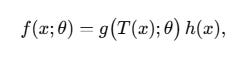
which just says that θ only ever “touches” the data through T. The sample mean is sufficient for the mean of a normal distribution. Knowing every individual observation buys you nothing beyond knowing their average. Fisher’s notion is a statement about information.

Economics kept Fisher’s word and changed its object, from parameters to counterfactuals. When an economist says “sufficient statistic,” she usually means sufficient for a welfare calculation or a policy counterfactual. The modern usage was codified by Raj Chetty in a 2009 review article with a subtitle that tells you exactly what the method is for: “A Bridge Between Structural and Reduced-Form Methods.” The idea had been building in public finance for years. Martin Feldstein had shown in the 1990s that to compute the deadweight loss of the income tax you do not need to separately model how people adjust their hours, their effort, their occupation, or their tax avoidance. You need a single number, the elasticity of taxable income with respect to the net-of-tax rate. All the behavioral margins that matter for efficiency are already summarized in how taxable income responds. Earlier still, Martin Baily (1978) had shown that the optimal level of unemployment insurance could be written in terms of just the drop in consumption a worker suffers on losing a job and the elasticity of unemployment duration with respect to benefits.

The structure of all these results is the same, and it is worth writing down because every macro result later in this essay is a variation on it:

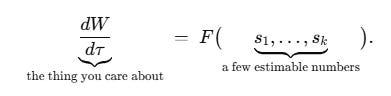
The welfare effect of a policy change, on the left, equals some formula, on the right, involving a small number of statistics you can estimate from data: elasticities, covariances, consumption drops. The structural primitives (utility functions, production technologies, the whole apparatus) have vanished from the right-hand side. That disappearance is what the method is selling.

But notice what Chetty himself was careful to say, and what a decade of enthusiasm sometimes forgot: the approach is not model-free. A different sufficient-statistic formula must be derived for each question, and deriving it requires taking a stand on the structure of the model. The formula F is only valid inside the class of models it was derived for. The primitives disappear from the formula because you assumed a class of environments in which their details cancel out. They still sit inside the derivation, doing work you have agreed not to examine. That qualification is the heart of the essay.

Three macro instances

Much of the canonical early sufficient-statistics work was developed in relatively partial-equilibrium policy settings. The hard and interesting move of the last fifteen years has been to carry the idea into full general equilibrium, into a setting where everything feeds back on everything else, and where the temptation to summarize is greater and more dangerous. Let me take three of the best examples, because seeing the pattern three times is what makes it visible.

One: aggregation, and Hulten’s revenge

Return to Hulten’s theorem, which I opened with. In an efficient economy, the elasticity of aggregate output to a productivity shock in sector i is that sector’s Domar weight, sales over GDP:

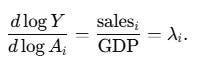
Notice what is absent from the formula. Nothing about the network, nothing about substitution or market power. One point will matter later: the Domar weight is itself an equilibrium object. It already encodes gross sales, input linkages, and intermediate flows. The network still matters in a deep sense. To first order, though, it does not enter separately once you know the sales shares, it is already folded into them. Those shares are a sufficient statistic for how micro shocks aggregate. Xavier Gabaix (2011) used a close cousin of this logic to argue that idiosyncratic shocks to the very largest firms, a “granular residual,” can drive a large share of aggregate volatility, because the firm-size distribution is so skewed that big firms never wash out in the average.

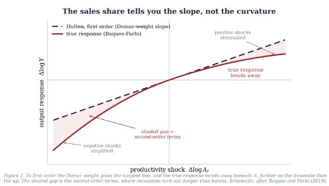
Now the bill. In 2019, David Baqaee and Emmanuel Farhi published a paper whose title is the warning: “The Macroeconomic Impact of Microeconomic Shocks: Beyond Hulten’s Theorem.” Their point is that Hulten’s sufficiency is a strictly first-order result, exact only for Cobb-Douglas economies, and only as a local approximation otherwise. Go to second order and every ingredient Hulten let you ignore returns: elasticities of substitution, the shape of the network, returns to scale, the extent to which factors can reallocate. And the second-order terms matter. They make the distribution of output asymmetric and fat-tailed even when the underlying shocks are symmetric and thin-tailed. Negative shocks get amplified, positive ones attenuated, so that recessions are endogenously deeper than booms are high. In their calibration, the output losses from business-cycle fluctuations come out roughly an order of magnitude larger than the near-zero welfare cost Robert Lucas made famous.

So the Domar weight is sufficient, for the linear response, in an efficient economy, to a small shock. Change any of those qualifiers and it is not. The sales share tells you the slope. It is silent about the curvature, and the curvature is where the disasters live. Figure 1 draws that gap: the tangent line is all Hulten gives you, and the true response bends away beneath it, further on the downside than the up.

Two: transmission, and the moment that matters

Second example. When a central bank cuts rates, or a government sends out checks, how much does spending respond? The textbook representative-agent answer uses one economy-wide marginal propensity to consume. But households differ, and which feature of that distribution is sufficient depends on the question you ask.

Adrien Auclert’s 2019 work on the “redistribution channel” of monetary policy makes this concrete. The extra consumption response, beyond the representative-agent benchmark, is captured by a set of covariances between MPCs and household balance-sheet exposures. The average MPC alone misses it. The clearest is the interest-rate exposure channel:

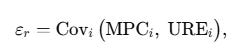
where UREᵢ, the unhedged interest rate exposure, is the difference between a household’s maturing assets and maturing liabilities. The logic is that a rate change redistributes between borrowers and savers, and this only moves aggregate spending if the winners and losers have different propensities to spend. Empirically the covariance is negative (high-MPC households tend to be borrowers), so heterogeneity amplifies monetary policy. Two more covariances, one for inflation exposure and one for income, complete the picture. Auclert traces the lineage of this move explicitly back to Harberger (1964) and Chetty (2009). It is the public-finance bargain, transplanted into monetary economics.

The deeper version of this idea is the “intertemporal Keynesian cross” of Auclert, Rognlie, and Straub (2024), where the sufficient statistic for the output response to fiscal policy grows into an entire matrix of intertemporal MPCs, how much you spend today out of income you expect to receive at each horizon in the future. Their empirical estimates are inconsistent with representative-agent and two-agent models, but can be matched by heterogeneous-agent ones, and they imply deficit-financed spending multipliers above one. Here the “few numbers” have become a whole object, but the philosophy is unchanged: pin down that object from micro data and you can compute the macro counterfactual without solving the full model.

The lesson repeats. The average MPC is sufficient for one question and insufficient for another. What you need is the joint distribution of propensities and exposures. The marginals will lie to you.

Three: policy evaluation, and the Lucas critique on a leash

Third example. Set welfare and aggregation aside: was a given policy decision actually good? The usual way to answer is to build a full structural model, which means taking a stand on almost everything. Barnichon and Mesters argued in 2023 that you need just two objects, and neither requires solving a fully specified structural model: the impulse responses of the objectives (say, inflation and unemployment) to policy shocks, and the central bank’s own conditional forecasts of those objectives.

Here is the reasoning. At an optimum, there is no predictable way to do better, so the gradient of the policymaker’s loss function with respect to a small policy change should be zero. That gradient is a weighted product of the two statistics, which makes the optimality condition a kind of orthogonality: your forecast of where the economy is headed should be uncorrelated with your ability to move it. When they correlate, you are leaving something on the table. Applied to US monetary policy, the optimal adjustments are usually small, around 25 basis points, with a few exceptions, the zero lower bound chief among them.

That is a lot of mileage from two estimable objects. But the catch is right there, and it is an old objection. The whole thing works only if the impulse responses you estimated under past policy behavior remain valid under the alternative policy you’re contemplating, that is, only if the private sector doesn’t re-optimize in response to the new rule. This is the Lucas critique, and the entire semi-structural literature (Barnichon and Mesters, but also McKay and Wolf (2023) on time-series counterfactuals, and Wolf’s (2023) “missing intercept”) is best understood as an effort to put the Lucas critique on a leash rather than pretend it has been solved. The move is to state the invariance assumption explicitly and only compute counterfactuals within its reach. That is real progress.

The pattern, and the sharper failure underneath it

Step back and the three examples rhyme. In each, a formidable structural object collapses to a few measurable numbers, and in each, that collapse is licensed by an assumption about the class of environments you’re willing to consider:

Hulten’s Domar weights are sufficient for the first-order response in an efficient economy.
Auclert’s covariances are sufficient for the first-order consumption response, within the class of models where those balance-sheet channels operate.
Barnichon and Mesters’ impulse responses are sufficient for policy counterfactuals in which the private sector is invariant to the perturbation.

The same shape appears far outside macro proper. In trade, Arkolakis, Costinot, and Rodríguez-Clare (2012) showed that the welfare gains from trade, across a range of models with different micro foundations, depend on just two numbers: the share of spending on domestic goods and the trade elasticity. Their title asks, drily, “New Trade Models, Same Old Gains?” and the answer is yes: conditional on the trade data, the micro details cancel. This is Hulten’s irrelevance wearing a different suit, and just as conditional. The moment you allow variable markups or non-CES demand, the two statistics stop being sufficient, and a literature grows up to handle each escape.

This much is the familiar half of the story. That a sufficient statistic is model-relative is what Chetty conceded and what Henrik Kleven (2021) drove home when he revisited the program. The selling point was “no structural model required.” Kleven shows how much that oversells. You can write sufficient-statistics formulas under very general conditions, but as you relax the assumptions the estimation requirements explode, and the feasible implementations turn out to be structural approaches in all but name. The theory has not gone away. It has been moved from the estimation stage, where you would have to defend it, to the derivation stage, where it sits silently inside the formula. An honest sufficient-statistic result always ships with its model class attached, the way a drug ships with its contraindications.

That is the familiar critique, and it does not go deep enough.

When sufficiency masks identification

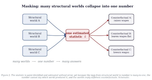
There is a failure mode underneath model-relativity, and it is the one I find most worth dwelling on, because it survives even when you have done everything right. The sufficient statistic can be right, and well estimated. The trouble is that a single statistic can collapse several structurally different worlds into one number, worlds that agree on the number and disagree on the counterfactual you actually care about. The problem is a many-to-one mapping from structure to summary. It has nothing to do with noise, and measuring the summary more precisely does nothing to break the tie. The statistic can be accurate and still hide the thing you need. Call that masking. Figure 2 is that collapse in one picture: several worlds funnel into one number, which fans back out to several answers.

Two things here are easy to conflate. The first is plain insufficiency: the statistic you reached for does not carry enough information, and a richer one would. Most of this essay has been about insufficiency, and insufficiency is the benign case. Baqaee and Farhi’s second-order terms are of this kind. The Domar weight is silent about curvature, so you go and measure elasticities of substitution as well. Auclert’s lesson has the same shape. The average MPC is too coarse, so you measure its covariance with exposure instead. In both cases the fix is to measure more, and the program absorbs the correction without complaint.

Masking is worse, because measuring more of the same statistic does not help. Here the statistic can be point-identified, estimated without error, and still fail to pin down the counterfactual, because the map from the structural world to the statistic is many-to-one. Two different economies produce the identical number and would respond differently to the policy. This is an identification failure sitting on top of a clean estimation. You can be perfectly right about the present and still wrong about the counterfactual, and no confidence interval will warn you, because the confidence interval is about the number, and the number is not where the ambiguity lives.

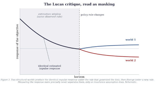
The sharpest case is hidden in one we have already met. Return to the policy-evaluation result. Barnichon and Mesters recover a set of impulse responses and treat them as sufficient for judging whether policy was optimal. Estimate those responses without error, and they are still consistent with several structural worlds that differ only in how much the private sector re-optimizes when the rule changes. Under the rule that generated the data, those worlds are observationally identical. Under the alternative rule you are weighing, they disagree. That is the Lucas critique, read as masking. The impulse response is a many-to-one shadow of the structures that could have produced it, and no confidence interval around it tells you which one you are in. Only a restriction does, the assumption that the private sector is invariant to the rule you are considering, and that restriction is exactly the structure the sufficient statistic promised to let you skip. Figure 3 shows the collision: the two responses coincide to the left of the rule change and separate to the right, one estimate, two counterfactuals.

The first two examples are milder failures: the missing object can be named, measured, and folded back into the statistic. The policy case is different. There, precision on the original number buys you nothing. Separating the structures takes new identifying restrictions, or new data that tell them apart. A tighter estimate of the same impulse response will not do it.

What to keep

I don’t want any of this to read as a debunking, because the sufficient-statistics program reshaped empirical macroeconomics for the better. Before it, the choice felt binary: either write down a full structural model and defend every assumption, or run a reduced-form regression that couldn’t answer the welfare or policy question you cared about. The sufficient-statistics move built a bridge, and it disciplined the conversation between the micro evidence economists can credibly estimate and the macro questions they actually want to answer. That is a considerable achievement, and the researchers I’ve cited are among the most careful in the field because they state their assumptions out loud.

The same warning applies wherever an exposure, an elasticity, or an impulse response is asked to do the work of a model.

A sufficient statistic is a bargain. You hand over the burden of estimating an entire structural model, and in return you get a formula in a few numbers you can measure. What you pay, always, is a set of assumptions about the class of models and the range of experiments over which that formula holds, and the price is easy to forget because it doesn’t appear on the right-hand side of the equation. Sometimes the price is that the formula holds only to first order. Sometimes it is that the same number could have come from a different world that answers your question differently. So when you meet a new sufficient statistic in the wild, the useful reflex is a question, the one this essay is named after, and the one that a perfectly estimated number can still fail to answer: sufficient for what?

Carlos Chavez

Discussion about this post

Ready for more?